Higher U.S. gasoline production and inventories are reducing gasoline crack spreads (6/15/2016)

Release date: June 15, 2016  |  Next release date: June 22, 2016

Higher U.S. gasoline production and inventories are reducing gasoline crack spreads

U.S. refiners are shifting their output mix to increase the gasoline production share and reduce the distillate production share, which is increasing gasoline inventories and beginning to reduce the gasoline crack spread—the difference between gasoline futures prices and crude oil. Monthly average gasoline crack spreads are now lower than they were last year, the second consecutive month of year-over-year declines. While distillate crack spreads are also lower than last year, they are only 3 cents per gallon (gal) lower than the five-year average and have increased 9 cents/gal over the past two months. Changing gasoline-to-distillate production ratios are a contributing factor in the difference in crack spreads.

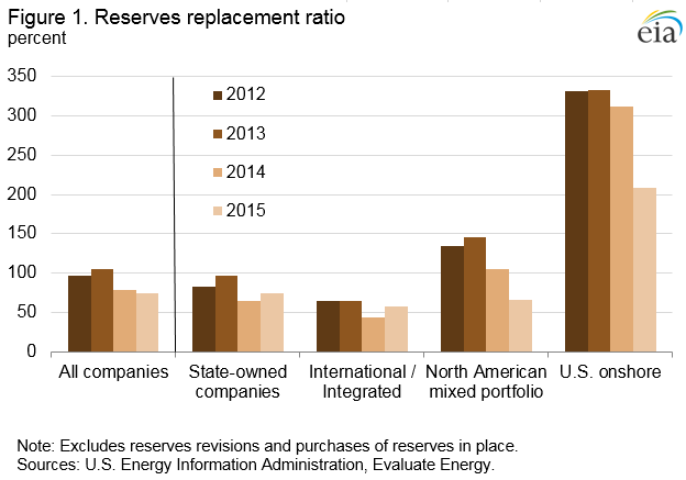
The U.S. gasoline-to-distillate production ratio began increasing in 2015, reversing a several-year decline. In May 2016, the gasoline-to-distillate production ratio reached a five-year high of 2.12 (Figure 1). Over time, refineries have some ability to adjust petroleum product yields in response to changes in price signals by adding additional equipment or modifying processes and feedstocks. A way for refineries to gauge product value is to look at the prices of futures contracts for delivery of a product at a future date. Because both gasoline and distillate prices exhibit seasonality in the summer and winter months, averaging the front-month and sixth-month futures contract price of each of the gasoline and distillate contracts and then calculating the price spread between the two averages provides insight into the price spread between these two physical products without reflecting sudden seasonal price swings that occur throughout the year.

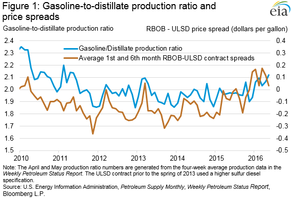
From 2010 to 2013, U.S. refineries increased production of distillate compared with gasoline because the average price of the New York Harbor distillate contract, which began trading ultra-low sulfur diesel (ULSD) in the spring of 2013, rose compared with the reformulated blendstock for oxygenate blending (RBOB, the petroleum component of gasoline) contract over that period. The strength in distillate prices was in response to rising distillate demand in developing countries, while U.S. demand for gasoline was stagnant or declining during much of that time.

However, in 2015, the trend changed, as the price of RBOB futures contracts rose compared with distillate contracts because of lower distillate demand and higher distillate inventories globally. Lower economic growth in developing countries and increased distillate exports from the Middle East and China led to high distillate stock levels in major storage hubs, including Singapore, northwest Europe, and the United States. On the other hand, the drop in crude oil prices in late 2014 was one of many factors that led to an increase in gasoline demand, both domestically and abroad. These developments spurred U.S. refineries to increase gasoline yields, which is contributing to the rise in overall U.S. gasoline production. In first-quarter 2016, total U.S. refinery and blender net production rose 0.82%, compared with the same period in 2015. During the same span, gasoline production rose 2.18%, while distillate production declined 2.56%.

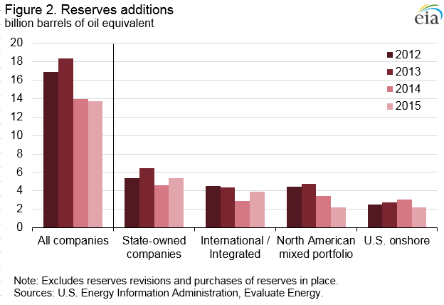
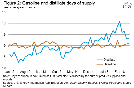
Inventories of both gasoline and distillate have been above the five-year historical range for most of 2016. As refineries increased gasoline production to meet rising demand, U.S. gasoline inventories leveled off after months of declines but are still well above the five-year range. On an absolute basis, gasoline inventories are 19 million barrels greater than at the same time last year and distillate inventories are also 19 million barrels higher. On days-of-supply basis, taking into account both domestic consumption and exports, U.S. gasoline inventories can fulfill an additional day of total gasoline demand than the same period last year (Figure 2). The year-over-year change in days of supply for gasoline gradually increased since February. Alternatively, the decline in distillate production and a slight strengthening of distillate demand following a very warm winter in the Northeast reduced the year-over-year change in distillate days of supply from a high of nearly 11 days in February to 3.2 days, according to the latest Weekly Petroleum Status Report.

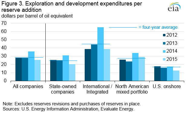
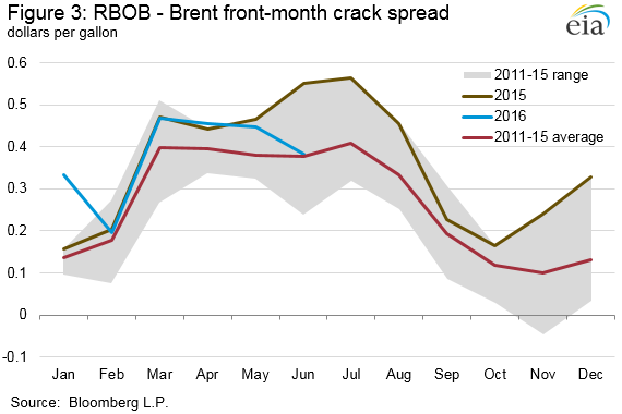
Despite an increase in gasoline consumption and exports so far this year over the comparable 2015 period, higher inventory levels are likely moderating price increases typically seen during the start of the summer driving season. Through June 14, the June 2016 average RBOB-Brent front month futures crack spread so far is 38 cents/gal compared with the June 2015 monthly average of 55 cents/gal last June (Figure 3). Unlike last spring and summer, when refineries were seeing gasoline crack spreads at their highest level since 2007, this year gasoline crack spreads may retreat closer to the average seen over the past five years.

U.S. average regular gasoline retail and diesel fuel prices increase

The U.S. average regular gasoline retail price rose two cents from the previous week to $2.40 per gallon on June 13, down 44 cents from the same time last year. The East Coast and Gulf Coast prices both decreased one cent to $2.31 per gallon and $2.14 per gallon, respectively. The Midwest price rose six cents to $2.47 per gallon. The West Coast price increased two cents to $2.72 per gallon. The Rocky Mountain price rose one cent to $2.32 per gallon.

The U.S. average diesel fuel price increased two cents to $2.43 per gallon, down 44 cents from the same time last year. The Midwest, Gulf Coast, and West Coast prices each increased three cents to $2.39 per gallon, $2.31 per gallon, and $2.71 per gallon, respectively. The Rocky Mountain price increased two cents to $2.41 per gallon. The East Coast price rose one cent to $2.45 per gallon.

Propane inventories gain

U.S. propane stocks increased by 1.1 million barrels last week to 78.4 million barrels as of June 10, 2016, 2.3 million barrels (2.9%) lower than a year ago. Midwest, Gulf Coast and Rocky Mountain/West Coast inventories increased by 0.7 million barrels, 0.6 million barrels, and 0.2 million barrels, respectively. East Coast inventories decreased by 0.4 million barrels. Propylene non-fuel-use inventories represented 4.3% of total propane inventories.

For questions about This Week in Petroleum, contact the Petroleum Markets Team at 202-586-4522.


Retail prices (dollars per gallon)

Conventional Regular Gasoline Prices Graph.On-Highway Diesel Fuel Prices Graph.
Gasoline 2.399 0.018 -0.436
Diesel 2.431 0.024 -0.439

Futures prices (dollars per gallon*)

Crude oil 49.07 0.45 -10.89
Gasoline 1.560 -0.048 -0.561
Heating oil 1.516 0.028 -0.373
*Note: Crude oil price in dollars per barrel.

Stocks (million barrels)

Crude oil 531.5 -0.9 63.6
Gasoline 237.0 -2.6 19.2
Distillate 152.2 0.8 18.6
Propane 78.351 1.057 -2.309

Storage capacity utilization rises, as growth in stored volumes outpaces expansion of storage capacity (6/8/2016)

Release date: June 8, 2016  |  Next release date: June 15, 2016

Storage capacity utilization rises, as growth in stored volumes outpaces expansion of storage capacity

The United States added 34 million barrels (6%) of working crude oil storage capacity from September 2015 to March 2016, the largest expansion of commercial crude oil storage capacity since EIA began tracking such data in 2011 (Figure 1). At the same time, reported weekly U.S. commercial crude inventories have increased by more than 72 million barrels (16%) since September, which implies crude oil storage capacity utilization at a record high of 74% for the week ending June 3.

Storage and capacity volumes used to calculate storage utilization rates must be comparable in scope to provide accurate estimates. Weekly U.S. crude inventories include volumes in transit by pipeline, tanker, barge and rail, and lease stocks. To facilitate accurate utilization calculations, EIA’s biannual Working and Net Available Shell Storage Capacity Report, which is released with March and September data, now provides information on the sum of working storage capacity, stocks in transit by pipeline, tanker, barge and rail, and lease stocks. This tally provides a capacity estimate with the same scope as commercial inventories reported by EIA for use as the denominator when calculating storage capacity utilization. Simply dividing total commercial inventories by working storage capacity alone would overstate utilization because it does not account for the volume of crude oil stored outside of tankage (pipeline fill and stocks in transit). Using weekly data, crude oil storage capacity utilization can be estimated by subtracting the amount of Alaskan crude oil in transit from commercial inventories, then dividing by the sum of working storage capacity, stocks in transit, and pipeline fill from the most recently available Working and Net Available Shell Storage Capacity Report.

The large increase in crude storage capacity between September and March was prompted by increased demand for crude oil storage as global supply has outpaced global demand for most of the past two years. Because of generally rising crude oil inventories since the end of 2014, the structure of crude oil futures prices has been in steep contango, where near-term deliveries are discounted versus long-term deliveries. The Nymex West Texas Intermediate (WTI) 1-13 spread averaged $7.25 per barrel between September and March. The large and continued contango structure prompted many market participants to place more crude oil into storage.

The largest commercial crude oil storage capacity expansions were in Petroleum Administration for Defense Districts (PADD) 2 (Midwest) and 3 (Gulf Coast), 19 million barrels (13%) and 13 million barrels (4%), respectively. Combined, PADDs 2 and 3 represent 82% of total U.S. commercial crude oil storage capacity. Within PADD 2, storage capacity at Cushing, Oklahoma, the delivery point for the Nymex WTI futures contract, expanded 1.5 million barrels (2%), similar to the previous period of March 2015 to September 2015, during which capacity expanded 1.6 million barrels (2%).

The expansion of crude oil storage capacity helped to accommodate the growth in U.S. crude oil inventories, which surpassed 500 million barrels at the end of January 2016. U.S. crude oil inventories increased in 24 of the 30 weeks from September to March, and were 532 million barrels for the week ending June 3.

Despite the large expansion in crude oil storage capacity, the net effect of capacity growth and increased inventories resulted in high storage utilization rates. Storage utilization at Cushing averaged 88% over the past four weeks, compared with 81% for the same period last year. PADD 3 storage utilization rates averaged 73% over the past four weeks, after having never surpassed 70% in the previous four years. (Figure 2).

U.S. average regular gasoline retail and diesel fuel prices increase

The U.S. average regular gasoline retail price increased four cents from the previous week to $2.38 per gallon on June 6, down 40 cents from the same time last year. The Midwest price increased seven cents to $2.41 per gallon, followed by the Gulf Coast, up five cents to $2.14 per gallon. The West Coast and East Coast prices each rose three cents to $2.70 per gallon and $2.31 per gallon, respectively. The Rocky Mountain price dipped slightly to $2.31 per gallon.

The U.S. average diesel fuel price increased three cents from a week ago to $2.41 per gallon, down 48 cents from the same time last year. The West Coast and East Coast prices each rose three cents to $2.68 per gallon and $2.44 per gallon, respectively. The Rocky Mountain, Midwest, and Gulf Coast prices each increased by two cents to $2.39 per gallon, $2.36 per gallon, and $2.28 per gallon, respectively.

Propane inventories gain

U.S. propane stocks increased by 1.9 million barrels last week to 77.3 million barrels as of June 3, 2016, 1.5 million barrels (1.9%) lower than a year ago. Gulf Coast, Midwest, and East Coast inventories increased by 1.4 million barrels, 0.5 million barrels, and 0.3 million barrels, respectively. Rocky Mountain/West Coast inventories decreased by 0.2 million barrels. Propylene non-fuel-use inventories represented 4.6% of total propane inventories

For questions about This Week in Petroleum, contact the Petroleum Markets Team at 202-586-4522.


Retail prices (dollars per gallon)

Conventional Regular Gasoline Prices Graph.On-Highway Diesel Fuel Prices Graph.
Gasoline 2.381 0.042 -0.399
Diesel 2.407 0.025 -0.477

Futures prices (dollars per gallon*)

Crude oil 48.62 -0.71 -10.51
Gasoline 1.608 -0.024 -0.422
Heating oil 1.488 -0.006 -0.382
*Note: Crude oil price in dollars per barrel.

Stocks (million barrels)

Crude oil 532.5 -3.2 61.9
Gasoline 239.6 1.0 22.3
Distillate 151.4 1.8 17.9
Propane 77.294 1.913 -1.501

Recent drilling activity has lowered costs and increased performance (6/2/2016)

Release date: June 2, 2016  |  Next release date: June 8, 2016

Recent drilling activity has lowered costs and increased performance

The profitability of oil and natural gas development activity depends both on the prices realized by producers and the cost and productivity of newly developed wells. Overall trends in well development costs are generally less transparent than those in price and productivity, which are readily observable in the markets or through analyses of well productivity trends such as EIA’s monthly Drilling Productivity Report.

To better understand the costs of upstream (or, wellhead) drilling and production activity, the U.S. Energy Information Administration (EIA) commissioned IHS Global Inc. (IHS) to study these costs on a per-well basis in the Bakken, Eagle Ford, and Marcellus plays, two plays within the Permian Basin (Midland and Delaware), and the offshore federal Gulf of Mexico (GOM). The IHS study finds that upstream costs in 2015 for the onshore plays were 25% to 30% below their 2012 levels, when per-well costs were at their highest point over the past decade, and 16% to 20% lower than the average of the past five years (Figure 1).

Changes in technology have improved drilling efficiency and completion, supporting higher productivity per well, but shifts toward deeper and longer lateral wells with more complex completions have tended to increase costs. To assess upstream costs of developing these plays in economic terms, the study applied the term unit cost, which compares capital expenditure with expected well performance to measure effectiveness, calculated as cost per barrel of oil equivalent (BOE) produced. Although some drilling costs have increased, the resulting performance benefit per well more than offsets those increases, leading to an overall decrease in cost per BOE produced (Figure 2). The unit cost concept does not, however, factor in the market value of the oil and gas produced from these wells, which is important for calculating net present value of profit or loss.

The use of multiwell pad drilling, more efficient fracturing and service providers, and decreased drilling times have all contributed to cost savings. At the same time, the use of longer laterals, better geo-steering to stay within the targeted formation, increased quantities of proppant use (to keep the fractured spaces open), an increased number and density of fracturing stages, and spacing optimization have increased well performance. Since oil prices started falling in mid-2014, reduced demand for drilling services has also enabled operators to renegotiate contracts with service providers, resulting in lower costs for drilling and well completions. Additionally, costs vary across the studied areas because of differences in geology, well depth, and water disposal options.

In the Bakken, lateral well lengths have increased to just under 10,000 feet to achieve a balance between cost and estimated ultimate recovery (EUR). Producers have also increased the quantity of proppant and fluids used at each stage, and a switch in the type of fracturing fluids. The type of proppant varies from expensive ceramic sand to cheaper natural sand between subplays, but is expected to move more toward natural sand. Well design and technology are expected to improve, but application of more proppant is not substantially increasing EURs, suggesting that as oil prices dropped in 2015, drilling operators switched to focusing on geological sweet spots rather than technological improvements to maintain production performance. Gathering, processing, and transport costs are high in this region because of infrastructure constraints associated with distance to markets and transportation being limited to rail (which can cost $5-$7 more per barrel than pipeline transport).

In the Eagle Ford, lateral lengths of wells have increased to 6,400 feet, while proppant and fracturing fluid quantities per stage have grown. Proppant mixes are focusing on cheaper, natural proppant allowing an economical increase of proppant. Also, more wells are being drilled on multiwell pads, allowing savings from shared facilities, roads, and water disposal systems. Unlike in the Bakken, an increased use of proppant directly correlates with production performance and abundant infrastructure, and proximity to markets decreases operating and transportation costs. Furthermore, in a low crude oil price environment, the Eagle Ford also has optimal production from site-specific drilling.

Horizontal wells in the Delaware and the Midland basins have increased their lateral lengths to 5,600 feet and 7,300 feet, respectively, with further increases projected. The Delaware Basin completion designs support 20 fractured stages with more than 6.2 million pounds of mixed natural sand and ceramic proppant and 6.6 million gallons of gel-based fluid. The Midland Basin designs support 28 stages with 8.8 million pounds of natural sand proppant and 9.2 million gallons of either slick water (low viscous fluid, mixture of water and chemicals) or gel-based fluid, with water-based fluid becoming more popular. However, even with these improving well and completion designs that have increased the EUR, sustained low prices have left unit costs in the Delaware Basin fluctuating and in the Midland Basin declining. Although horizontal wells in these basins have diminished cost savings in recent years, the Midland Basin is projected to have as many as 24 horizontal wells drilled from a single pad, potentially reducing costs by $700,000 per well. Similarly, horizontal drilling in the Delaware is expected to see incremental efficiency gains as more wells are drilled from multiwell pads.

Offshore projects are typically more complex than onshore ones, as they can require construction and installation of infrastructure unique to the project, and take years to develop. There are fewer wells from which to examine historical and current costs and a larger variation in the costs themselves. To demonstrate the variability in project costs, the IHS study characterized the cost profiles of four deepwater GOM projects representing the different plays, development concepts, and technical challenges offshore operators encounter: Chevron’s Big Foot ($4.3 billion), Anadarko’s Lucius ($2.47 billion), Deep Gulf Energy’s Kodiak ($1.2 billion), and Chevron’s Jack/St. Malo ($12 billion). Jack/St. Malo came online in 2014 and Lucius in 2015; Kodiak and Big Foot are anticipated to come online in 2016 and 2018, respectively.

The study delineated the main cost components of offshore projects and analyzed the key drivers behind each. The costs of drilling and completing wells in deepwater are driven by water depth, well depth, and reservoir quality, complexity, and productivity. The costs associated with constructing and installing the selected development concept are driven by design, reserve size, water depth, technical challenges, and infrastructure availability or proximity. The costs of laying pipeline used to transport processed oil and natural gas to an existing platform or onshore facility are driven by water depth, length, diameter, and capacity. Finally, the operating and decommissioning costs depend on the development concept.

Looking to 2018, with the significant capital investment offshore projects require and the current oil price environment, offshore operators are especially focused on reducing costs, increasing efficiency, and improving project economics. The IHS study estimates that a reduction in capital expenditure of at least 20% is required to move yet-to-be-funded projects in the most technically challenging play in the GOM to a $60/barrel breakeven. The study forecasts a 15% reduction in deepwater costs in 2015, an additional 3% reduction in 2016, and a modest rise in costs from 2017 to 2020.

U.S. average regular gasoline retail and diesel fuel prices rise

The U.S. average regular gasoline retail price increased four cents from the previous week to $2.34 per gallon on May 31, down 44 cents from the same time last year. The Midwest price increased six cents to $2.34 per gallon, followed by the East Coast, up four cents to $2.29 per gallon, and the Gulf Coast price, which rose three cents to $2.09 per gallon. The West Coast and Rocky Mountain prices each increased two cents to $2.67 per gallon and $2.32 per gallon, respectively.

The U.S. average diesel fuel price increased three cents from a week ago to $2.38 per gallon, down 53 cents from the same time last year. The West Coast price rose five cents to $2.65 per gallon, followed by the East Coast price, which increased three cents to $2.41 per gallon. The Rocky Mountain, Midwest, and Gulf Coast prices each increased two cents to $2.38 per gallon, $2.34 per gallon, and $2.25 per gallon, respectively.

Propane inventories gain

U.S. propane stocks increased by 1.3 million barrels last week to 75.4 million barrels as of May 27, 2016, 1.7 million barrels (2.2%) lower than a year ago. Midwest and Rocky Mountain/West Coast inventories increased by 1.3 million barrels and 0.2 million barrels, respectively. Gulf Coast inventories decreased by 0.3 million barrels, while East Coast inventories remained virtually unchanged. Propylene non-fuel-use inventories represented 5.1% of total propane inventories.

For questions about This Week in Petroleum, contact the Petroleum Markets Team at 202-586-4522.


Retail prices (dollars per gallon)

Conventional Regular Gasoline Prices Graph.On-Highway Diesel Fuel Prices Graph.
Gasoline 2.339 0.039 -0.441
Diesel 2.382 0.025 -0.527

Futures prices (dollars per gallon*)

Crude oil 49.33 1.58 -10.97
Gasoline 1.632 -0.004 -0.454
Heating oil 1.494 0.004 -0.461
*Note: Crude oil price in dollars per barrel.

Stocks (million barrels)

Crude oil 535.7 -1.4 58.3
Gasoline 238.6 -1.5 18.3
Distillate 149.6 -1.3 17.0
Propane 75.381 1.252 -1.665

Oil companies focus on production over exploration as low oil prices reduce value of new reserves (5/25/2016)

Release date: May 25, 2016  |  Next release date: June 2, 2016

Oil companies focus on production over exploration as low oil prices reduce value of new reserves

For the second consecutive year, oil companies worldwide produced more oil and natural gas than they added to their proved reserves, excluding revisions to existing proved reserves and purchases of reserves in place. This is not necessarily an indication of fewer available resources, but rather that at current prices, there are fewer resources that can be turned into proved reserves, which are underground oil and gas that can be commercially produced at current prices using currently available technology.

Based on analysis of recently released annual reports, 85 publicly traded companies added a total of 13.7 billion barrels of oil equivalent (BOE) to their reserves base, three-quarters of the amount the same group of companies produced in 2015. A combination of reductions in exploration and development (E&D) investment and fewer extensions and discoveries contributed to the decline. Of the companies that submitted first-quarter 2016 financial results, capital expenditures declined 35% from first-quarter 2015, suggesting continued reductions in E&D investment, which could reduce reserves additions in 2016.

The reserves replacement ratio—the ratio of proved reserves added during a given year to production for that year—indicates the extent to which a company is replacing its produced reserves (Figure 1). The group of 85 companies as a whole had a reserves replacement ratio of approximately 100% in 2012 and 2013, and around 75% for 2014 and 2015. However, the ratios vary significantly by company type. Only the U.S. onshore companies added more reserves to their collective portfolio than they produced in 2015, but the effect on the global reserves base is modest because these companies hold a relatively small share of proved reserves and production.

Each company grouping differs by its area of operations and the types of assets in its portfolio. State-owned companies are mostly national oil companies outside of the Organization of the Petroleum Exporting Countries (OPEC). The international/integrated oil companies are large producers that have refining and midstream assets, with global portfolios of onshore and offshore oil production. The North American mixed companies are U.S. and Canadian exploration and production (E&P) companies that are smaller producers but with fairly broad portfolios geographically and by production type, including shale, oil sands, and offshore. The U.S. onshore producers are smaller E&P companies that focus mainly on onshore production in the United States. Collectively, the 85 companies produced 50 million BOE per day in 2015, two-thirds of which was crude oil and the remainder being natural gas and hydrocarbon gas liquids.

Analysis by major area of operations and production portfolio also reveals volumetric differences in reserves additions (Figure 2). State-owned companies and international/integrated oil companies increased reserves additions in 2015, while North American companies with a mixed production portfolio and U.S. onshore companies added less than in 2014. Companies can add proved reserves through new discoveries, enlargement of a reservoir’s proved area (extensions), improvements in the recovery of existing reserves, purchases of another company’s proved reserves, or revisions of existing reserves for economic or technical reasons. For the purposes of this analysis, purchases of reserves in place and reserves revisions are excluded from the calculation of reserves additions.

Expenditures for E&D constitute most of a company’s upstream capital investment. When calculated on a reserve addition per barrel basis, these expenditures represent the cost of finding and developing a barrel of oil. Finding and developing costs declined $10.23/BOE in 2015 (Figure 3). Since there may be a timing mismatch between when an expenditure is made and when a proved reserve addition is formally recognized, standard practice is to average the results over several years. Finding and developing costs for these companies were $25.69/BOE in 2015, the lowest in the 2012-15 period and lower than the four-year average of $29.25/BOE.

Similar to the reserves additions and the reserves replacement ratio, finding and developing costs differed across the company groupings. In recent years, U.S. onshore companies tended to have lower E&D expenditures per reserve addition compared with the other groups, as many reserves additions came from geologically familiar shale basins in the United States. Other producers typically operate in areas where it is more challenging to find reserves, such as deepwater offshore or in more mature fields that are the foundation of legacy production (such as in China or Russia). The decline in E&D expenditures for national oil companies and international/integrated companies suggests a reduction in exploration activity in such high-cost areas.

With most companies indicating continued reductions in E&D budgets absent a meaningful increase in crude oil prices, proved reserves additions will likely continue to decline.

U.S. average regular gasoline retail and diesel fuel prices increase

The U.S. average regular gasoline retail price increased six cents from the previous week to $2.30 per gallon on May 23, down 47 cents from the same time last year. The Midwest price increased 10 cents to $2.28 per gallon, followed by the Gulf Coast, up eight cents to $2.06 per gallon. The Rocky Mountain price rose six cents to $2.30 per gallon, the East Coast price increased three cents to $2.25 per gallon, and the West Coast price rose one cent to $2.66 per gallon.

The U.S. average diesel fuel price increased six cents from a week ago to $2.36 per gallon, down 56 cents from the same time last year. The Gulf Coast price rose eight cents to $2.23 per gallon, followed by the West Coast price, which increased seven cents to $2.60 per gallon. The East Coast price increased six cents to $2.38 per gallon, the Midwest price rose five cents to $2.33 per gallon, and the Rocky Mountain price was up three cents to $2.36 per gallon.

Propane inventories fall slightly

U.S. propane stocks decreased by 0.1 million barrels last week to 74.1 million barrels as of May 20, 2016, 0.9 million barrels (1.2%) higher than a year ago. East Coast and Gulf Coast inventories decreased by 0.2 million barrels and 0.1 million barrels, respectively. Midwest inventories increased by 0.2 million barrels, while Rocky Mountain/West Coast inventories remained unchanged. Propylene non-fuel-use inventories represented 5.4% of total propane inventories.

For questions about This Week in Petroleum, contact the Petroleum Markets Team at 202-586-4522.


Retail prices (dollars per gallon)

Conventional Regular Gasoline Prices Graph.On-Highway Diesel Fuel Prices Graph.
Gasoline 2.300 0.058 -0.474
Diesel 2.357 0.060 -0.557

Futures prices (dollars per gallon*)

Crude oil 47.75 1.54 -11.97
Gasoline 1.636 0.048 -0.418
Heating oil 1.490 0.087 -0.463
*Note: Crude oil price in dollars per barrel.

Stocks (million barrels)

Crude oil 537.1 -4.2 57.7
Gasoline 240.1 2.0 19.5
Distillate 150.9 -1.3 22.0
Propane 74.129 -0.087 0.911

Clean Power Plan accelerates the growth of renewable generation throughout United States

June 17, 2016graph of U.S. net electricity generation by fuel, as explained in the article text


EIA’s Annual Energy Outlook 2016 (AEO2016) Reference case projects that natural gas-fired electricity generation will exceed coal-fired electricity generation by 2022, while generation from renewables—driven by wind and solar—will overtake coal-fired generation by 2029. The shift away from coal-fired generation to a combination of higher natural gas-fired and renewables generation and greater energy efficiency is expected to be accelerated by the U.S. Environmental Protection Agency’s Clean Power Plan (CPP).

Notably, the share of natural gas-fired generation exceeded coal-fired generation in 2016, according to EIA’s latest Short-Term Energy Outlook. However, in the AEO2016 Reference case, the natural gas-fired share of generation declines temporarily after 2016, then resumes rising in about 2020 and once again exceeds the coal-fired share in 2022 and throughout the rest of the AEO2016 projection to 2040.

Even without the CPP, significant growth in renewables generation is projected throughout the country, due in large part to Congress’s recent extension of favorable tax treatment for renewable energy sources. From 2015 to 2030, for the nation as a whole in a scenario where the CPP is never implemented, EIA projects that renewables generation will increase at an annual average rate of 3.9%, while natural gas generation will grow at 0.6% per year. In the Reference case, which assumes the implementation of the Clean Power Plan, renewables and natural-gas fired generation grow at 4.7% and 1.6% annually from 2015 to 2030, respectively.

In the final version of the CPP, states with higher intensity levels generally have greater requirements for reduction of CO2 emissions.

graph of electricity market regions and carbon dioxide emissions rate by region, as explained in the article text


EIA’s analysis of the U.S. electricity market is divided into 22 regions, which in this discussion are further reduced to 9 regions shown above. The current generation mix across these regions varies considerably, with significant differences in the use of fossil-fuel, nuclear, and renewable energy sources.

graph of regional electricity generation by fuel, as explained in the article text


Certain regions such as the Midwest/Mid-Atlantic, Southwest/Rockies, and Northern Plains—regions that are home to much of U.S. coal production—tend to have greater reliance on coal-fired electricity generation. These regions have among the highest CO2 reduction requirements and are expected to have the largest shifts in their generation mix. In the Midwest/Mid-Atlantic region, a large decline in coal generation is offset by an increase in natural gas generation and relatively modest growth in renewable generation. These projected changes are expected to result in a 26% decline in the Midwest / Mid-Atlantic region’s emission rate—from 1,826 to 1,357 pounds of CO2 per megawatthour, the largest drop of any region in both percentage and absolute terms.

The Southwest/Rockies region is projected to see an expansion of renewables generation that is nearly twice as large as the decline in coal generation. In the Northern Plains region, a decline in coal generation is exceeded by a slightly larger shift to renewables generation, with smaller growth in natural gas generation. Other regions, such as Texas, the Southern Plains, and the Southeast, rely more on natural gas-fired generation. The projected decline in these regions’ coal generation is more modest, and they all are expected to see strong gains in renewables generation, with some additional growth in natural gas generation.

Finally, the Northeast region and California currently have almost no coal generation and meet most of their demand with natural gas generation, along with renewables generation in California and a mix of nuclear and renewables generation in the Northeast. While the Northwest region does have some coal generation, it has the largest renewable generation total of any region because of its extensive hydroelectric resources. These regions have among the lowest emission reduction requirements, and as a result are expected to register small or no change in generation mix as a result of the CPP.

California sees strong growth in renewable generation by 2030 as a result of the state renewable targets. Similarly, the Northwest region is expected to increase renewables generation as well. The Northeast shows an increase in both natural gas and renewables generation by 2030, and a small decline in nuclear generation due to planned retirements.

The Reference case assumes that all states implement the Clean Power Plan using a mass-based standard that caps emissions from both existing and new plants, with allowance revenues rebated to rate payers. Because the plan allows flexibility in implementation approaches, EIA produced several alternative cases that consider how outcomes change with different implementation approaches, and in a scenario with tighter standards beyond 2030. Compliance decisions by the states (as well as any future court decision that would vacate the rule) have implications for plant retirements, capacity additions, and generation by fuel type, demand, and prices. An AEO2016 Issues in focus article released early next week will explore the results of this analysis.

Principal contributors: Thad Huetteman, Laura Martin

Measuring the value of next-generation wind and solar power

As next-generation wind and solar power grows in the energy mix, a focus on their falling generation costs alone stops short of what is needed

2 June 2016

In a paper released today on the side-lines of the Clean Energy Ministerial in San Francisco, the International Energy Agency argues that a new phase of deployment in wind and solar photovoltaics (PV) – currently the fastest-growing sources of electricity globally – is emerging, in which wind and solar PV are technologically mature and economically affordable. However electricity generation from both technologies is constrained by the varying availability of wind and sunshine, which can make it more difficult to maintain the necessary balance between electricity supply and consumption.

As these variable renewables enter this next generation of deployment, the issue of system and market integration becomes a critical priority for renewables policy and energy policy more broadly. The paper highlights that this will require strategic action in three areas:

• System-friendly deployment, aiming to maximise the net benefit of wind and solar power for the entire system
• Improved operating strategies, such as advanced renewable energy forecasting and enhanced scheduling of power plants
• Investment in additional flexible resources, comprising demand-side resources, electricity storage, grid infrastructure and flexible generation

In addition, the paper argues that unlocking the contribution of system-friendly deployment calls for a paradigm shift in the economic assessment of wind and solar power. The traditional focus on the levelised cost of electricity (LCOE) – a measure of cost for a particular generating technology at the level of a power plant – is no longer sufficient. Next-generation approaches need to factor in the system value of electricity from wind and solar power – the overall benefit arising from the addition of a wind or solar power generation source to the power system. System value is determined by the interplay of positives and negatives including reduced fuel costs, reduced carbon dioxide and other pollutant emissions costs, or higher costs of additional grid infrastructure.

In addition to general analysis and recommendations, the paper also includes summaries of three case studies in China, Denmark and South Africa..

Next-Generation Wind and Solar Power: from Cost to Value
is available for free download here.


Total U.S. electricity sales projected to grow slowly as electricity intensity declines

June 15, 2016graph of electricity sales by sector, as explained in the article text


Electricity sales, as projected in the U.S. Energy Information Administration’s most recent Annual Energy Outlook (AEO2016) Reference case, increase in each sector through 2040. In 2015, 3.7 trillion kilowatthours (kWh) of electricity were sold, and total electricity sales are projected to rise 0.7% annually through the projection period. The residential sector currently purchases the most electricity, with a 38% share of total electricity sales in 2015. However, sales in the commercial sector are projected to surpass those in the residential sector in the early 2020s.

The AEO2016 Reference case, which reflects current laws and regulations, includes the U.S. Environmental Protection Agency’s Clean Power Plan (CPP). The CPP allows state regulators to encourage customers to purchase specified energy-efficient technologies as a part of state compliance strategies. The AEO2016 Reference case assumes that consumers will receive subsidies of 10% or 15% between 2020 and 2025 for certain energy efficient appliances, equipment, and building envelope improvements.

graph of residential, commercial, and industrial energy intensity, as explained in the article text


The residential sector currently is the largest electricity-consuming sector, with 1.4 trillion kWh sold in 2015. Electricity sales in the residential sector are projected to grow by 0.3% per year in the Reference case from 2015 through 2040 as the number of households increases by 0.8% per year. Residential energy intensity is expected to decline, with the average purchased electricity per household falling 11.3% from 2015 to 2040. Federal efficiency standards for most major end uses, including lighting, space cooling and heating, and water heating, as well as state and local building energy codes, are the main reasons for the electricity intensity decline.

Electricity sales to commercial consumers are projected to increase at an average annual rate of 0.8% from 2015 to 2040. Commercial sector electricity intensity (electricity sales per square foot of floorspace) is projected to decline 0.3% per year as total commercial sector floorspace increases 1.1% per year. Federal energy efficiency standards, as well as technological improvements in lighting, refrigeration, space heating, and space cooling, contribute to the decline in electricity intensity.

Electricity sales to industrial consumers are projected to rise 1.1% per year on average, from 1.0 trillion kWh in 2015 to 1.2 trillion kWh in 2040. With the value of industrial shipments projected to grow 1.9% per year in the Reference case, industrial sector electricity intensity, or electricity sales per dollar of industrial shipments, declines at an average annual rate of 0.8% from 2015 to 2040. The decline in projected electricity intensity results from the adoption of more energy-efficient technologies and structural changes in the economy toward less electricity-intensive industries.

A recent extension of federal tax credits for residential and commercial solar photovoltaic (PV) systems, combined with the expected continuation of declining PV prices, spurs increased adoption of residential and commercial PV in the AEO2016 Reference case projection. Total building PV capacity grows at 8.6% annually in the AEO2016 Reference case. Generation from residential PV systems reaches 90 billion kWh, and commercial system generation reaches 36 billion kWh by 2040. Residential and commercial electricity sales would be 5.0% and 1.7% higher, respectively, in 2040 without the electricity generated by rooftop PV systems.

Principal contributor: Kimberly Klaiman